The Power Transfer Capability of Transformers

On a Friday afternoon, I was about to go home from the office when the phone rang. A customer asked an interesting question. This stems from a 30VA 50Hz transformer that we had designed for him, but which is actually being used in a 40VA application. “So what impact would this running situation have on the transformer,” said the client engineer at the other end of the line?

Knowing the design of the transformer, its power rating definitely can be increased to 40VA with obviously the biggest impact being an additional temperature rise of about 10°C and a slight output voltage drop at full load. The reason is, of course, that the output load is increased. The engineer carried on, “If we don’t take the temperature rise into account, is it correct to assume that the power of this transformer can be infinitely increased?” Listening to his conjecture on potentially infinitely increasing the transformer power transfer, I blurted out, “that is impossible, the power of the transformer will overflow ( a so called “power overflow”), like the coffee in a coffee cup will overflow because the cup has a finite volume capacity.”

This problem, in fact, is about the transformer’s power transfer capability. To address this question, a good start is from a transformer equivalent circuit. In theory, the ideal power transformer is a device that neither produces, stores, nor consumes any energy. It only transfers the power from the power network to the load by changing the primary and secondary voltage in accordance to the fixed turns ratio. However, in reality, due to the intrinsic losses of iron cores (core loss) and the presence of winding resistance (copper loss), the power of the transformer is not 100% transferred, so the input and output voltage of the transformer is not a simple relationship of turns ratio. This can be explained from the dual port equivalent circuit of the transformer shown in Fig. 1 below.

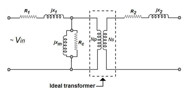
Where Vin is the input power supply voltage, R1 is the transformer primary winding resistance, X1 is the transformer primary leakage reactance, Rc is the transformer core loss equivalent resistance, Xm is the transformer excitation reactance. R2 is the transformer secondary winding resistance, X2 is the transformer secondary leakage reactance.

As long as the primary is connected to a voltage source, the secondary winding of the transformer will induce an output voltage. When the transformer is under no-load conditions, even the secondary circuit is open, there is a loop in the primary circuit, resulting in a current flow through the primary circuit. This current is called “the no load current”. Generally speaking, the equivalent core resistance Rc will be much larger than the transformer reactance Xm ( i.e. Rc >> Xm ), so the transformer no-load current can be considered as the transformer excitation current. It is this excitation current that establishes the working magnetic field of the transformer (denoted with flux density B), and achieves its function of changing the output voltage.

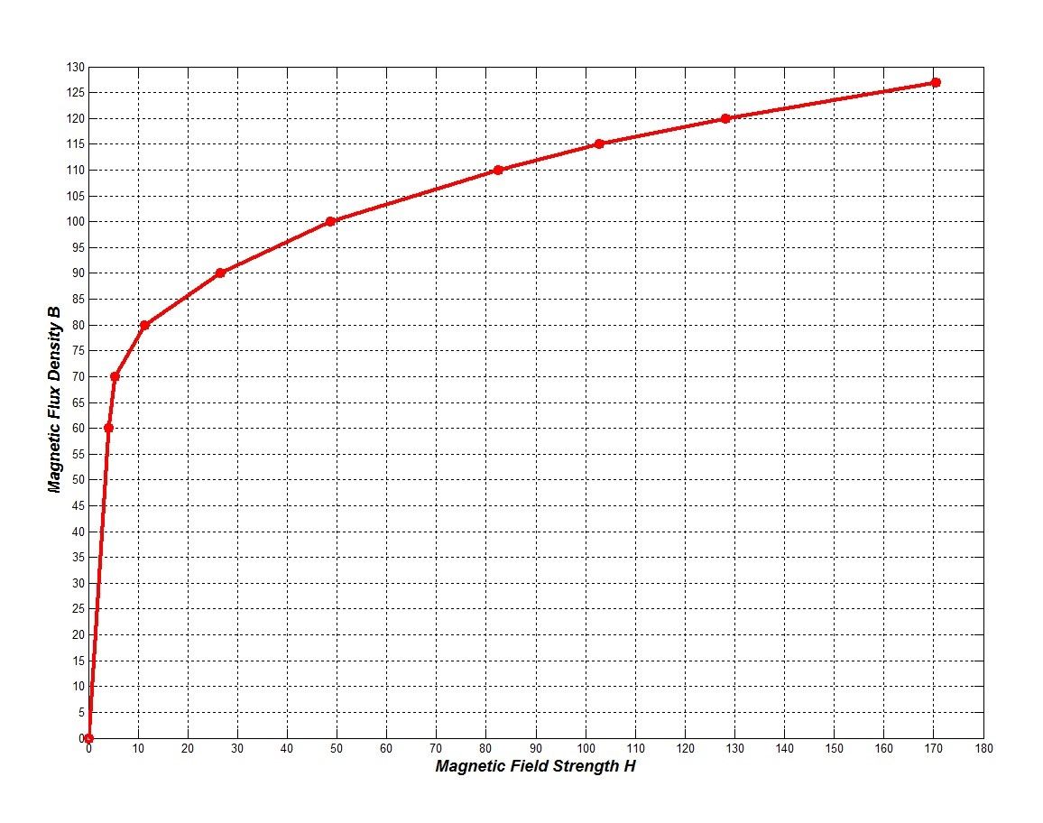
(This curve is derived from practical results and is slightly different from the theoretical result)

This B-H curve can be divided into three sections. The first of these being the magnetic loss compensation stage, followed by the rapid flux increase segment in the middle, and finally the magnetic flux saturation region, i.e. the portion of the B-H curve that is bent to the right. When the transformer excitation current is very small, it produces the magnetic field strength H applied to the core; the core is then magnetized, and magnetic field produced accordingly is not strong. In this stage, the B-H curve changes gently. When the field current increases, the core is magnetized to produce a rapid increase in magnetic flux. Therefore, the B-H curve at this stage is very steep. When the excitation current of the transformer increases to a certain level, the change of the magnetic field strength ∆H is much larger than that of the change of the magnetic flux density ∆B. This means the transformer core reaches saturation. At this stage, the B-H curve becomes flat.

As a transformer design engineer, if we design a transformer within the power rating given by the customer, the last thing we want to design is a large and bulky transformer to meet the performance requirements. We look at the trade-offs to get an optimised balance between the performance, it’s size and it’s manufacturability as well as other factors. Therefore, each transformer should be designed as close as possible to its maximum power transfer capability, with a reasonable temperature rise. In order to maximize the use of core materials, it is important to select the rated working magnetic induction density B as close to the tail of second stage of the B-H curve as possible, where the curve begins to turn horizontally.

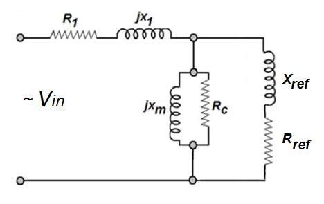
Figure 3 shows the equivalent circuit of a transformer, in the loaded condition, with the secondary circuit reflected to the primary circuit under the loaded condition. In general, for a 50Hz step down transformers, the input voltage is the mains voltage, varying from 100V to 240V, so the number of turns in the primary winding is large. Therefore, the value of the excitation reactance Xm is much larger, compared to the secondary reflected impedance to the primary side. If the input voltage does not change, ignoring the voltage drop caused by the primary winding impedance, the excitation current will remain unchanged. At the same time, the current of the primary side also increases as it will transfer enough energy to the load. In other words, the increased current in the primary current is used to balance the current generated by secondary load.

It has been said earlier that an ideal transformer is a device that neither produces, stores nor consumes energy. The transformer can be regarded as a power / energy transmission pipeline. If the load is infinitely increased (as the customer engineer has proposed), the current on the primary side increases as the secondary current increases. The voltage drop on the primary winding will increase accordingly. It is worth noting that the voltage actually loaded into the field excitation circuit is reduced, and the actual transformer magnetizing current is getting lower; and the secondary induced voltage also becomes smaller. At the same time, the voltage drop of the secondary winding becomes larger, resulting in a significant reduction in the load voltage. These changes can be clearly seen in Fig.4.

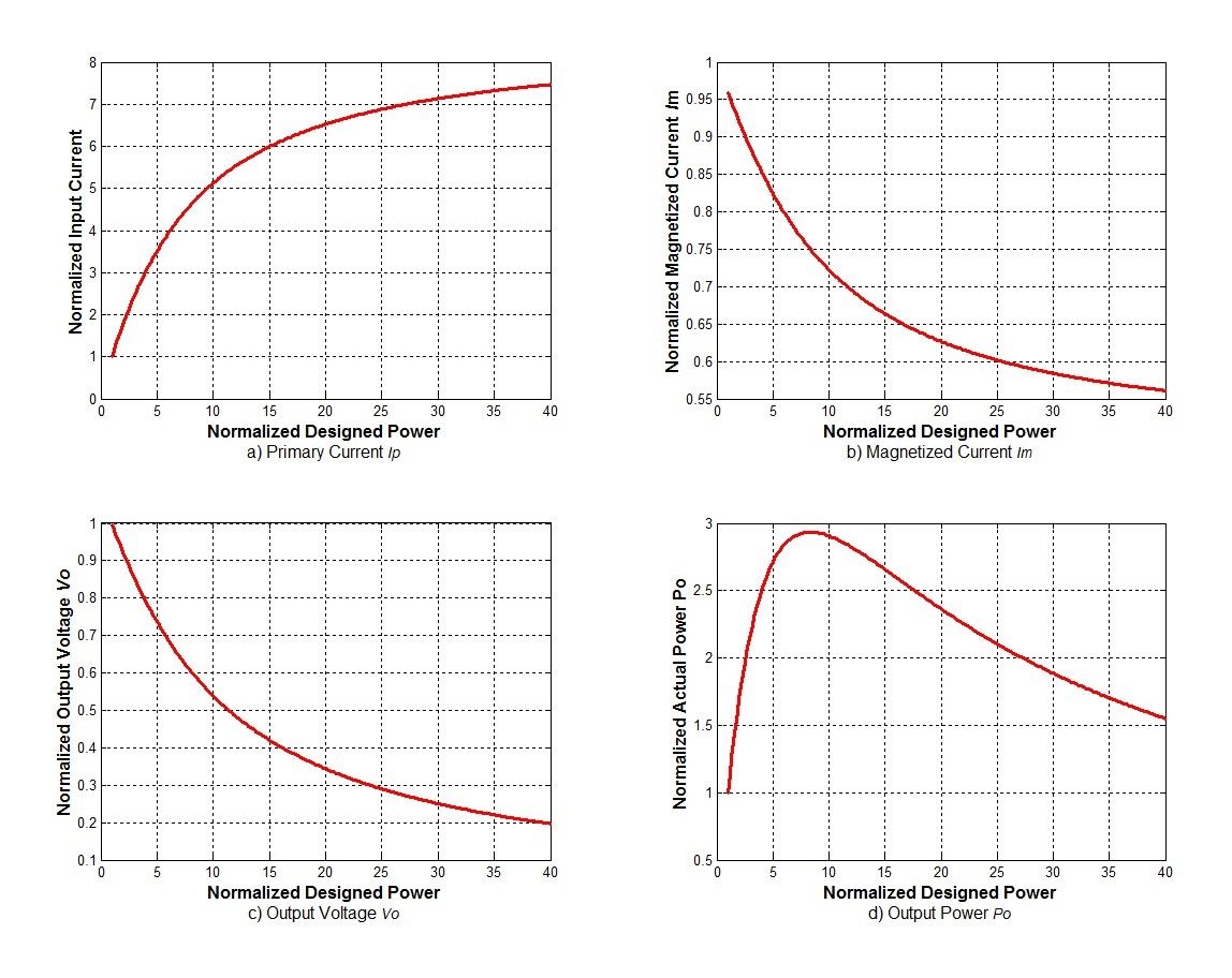
It is assumed a transformer is to deliver a power of four times more than the original rated power, i.e. the output dummy resistor is 1/5 of the nominal load value. From Fig. 4 a), it shows that the input current of the transformer is now increased by 2.5 times of the rated current, while in Fig. 4b), the excitation current is as low as 87% of the original excitation current; At the same time, the actual output voltage of the transformer is reduced to 75% of the original design voltage, as shown in 4c). The actual output power, however, is supposed to be increased to 5 times the rated power, in fact it gains only 2.7 times the rated output power. This can be clearly seen in Fig. 4d) where there is a maximum point in the power transfer curve. When the desired power exceeds 7 times the rated power, the transformer reaches the maximum power transfer capacity. However, the actual maximum transferred power is only about 3 times of the rated power. This is what we call “the power overflow” mentioned earlier in this article. This means that once the core size of the transformer is determined, its maximum power transfer capability is also determined and predictable.

It is important to point out here that what dominates the saturation level of a transformer core is not the current, but the input voltage. In the transformer designing stage, it is essential to properly choose the maximum magnetic flux density B from the B-H curve of the core characteristics provided by the suppliers. Bear in mind that the transformer input voltage determines the transformer core loss, and the transformer current dominates the transformer copper loss.

When the transformer core loss is constant, increasing the transformer current means increasing the transformer copper loss at the same time. This accelerates the increase of the transformer temperature rise. Due to the presence of copper loss, it constrains the unlimited increase of the transformer transfer power.

In general, the rule of thumbs to design an 50Hz transformer is to carefully select the appropriate magnetic flux density B to ensure that the transformer does not saturate. Secondly, choose the proper winding wire gauge to allow the transformer temperature rise to be within a reasonable range for the transformer application, as well as to optimize energy consumption. As sustainable development is the new norm today, this requires a design engineer to consider these rules when doing design planning.